Image primer
We are surrounded by images, all day, every day. We copy, paste, swipe, snap, share, ... But working with mission images, we have to reset our minds to a different approach. This deep dive is all about working with image data products from the PDS archive.
Who doesn't like looking at pictures from other worlds? How amazing! That amazing picture you see on a web page has a complex ancestor: a science data file with a format that most computer programs don't understand. Instead, you have to use specialized software to work with archive images because the information in images often cannot be stored in everyday formats like JPEG.
Sometimes you will find a browse version of an image that can be opened in a web browser or pasted into your presentation. This is a simplified version of an image that is useful for quickly assessing an image, but it is not suitable for containing the detailed science measurements. Browse versions, also called quicklooks, generally are not suitable for science-based research.
Image structure
All images share common attributes regarding their size: samples, lines, and bands.
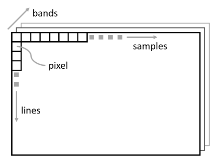
- A pixel is an individual "dot" in the image. In the data file, each pixel has a numeric value—the higher the value, the brighter the pixel when the image is displayed.
- Samples and lines are given in the number of pixels. Each row has the same number of samples, and each column has the same number of rows.
- An image has one or more bands of data collected at specific wavelengths as part of the same observation. You might have seen a color photo separated into its red, green, and blue components, each of which can be thought of a separate image band. All bands in an image have the same number of samples and lines whether there is one band or a hundred.
Some images have more complex structures, but this is a good place to start.
Going extra deep on data types
Data interleave
A computer program reads the pixel values from an image file as a sequence of numbers.
![]()
It needs to know the image structure, specifically the number of samples, lines, and bands, and in what order to expect the pixels—the data interleave. Three common data interleaves found in image processing software are band sequential (BSQ), band interleaved by pixel (BIP), and band interleaved by line (BIL).
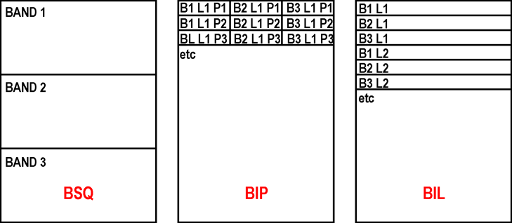
In band sequential order, all of the pixels for each band are in a contiguous block: [sample 1, line 1, band 1] [sample 2, line 1, band 1] [sample 3, line 1, band 1] and so on to the end of the first line, then on to the second line, third line, etc. Once we are at the end of the first band, the next pixel will be [sample 1, line 1, band 2]. If you consider the image as a three dimensional cube with samples, lines, and bands as the three axes, the sample axis is changing the fastest. You can imagine other arrangements of pixels in an image. So can the data providers.
Pixels data types
Each image pixel in a data file has a numeric value, and for any image the pixel values will fall within a certain range, for example integers from 0 to 255. Some images have pixel with real (floating point) number values or that span a larger range of values. Assigning a data type to an image constrains the pixel values allowed. A "byte image" is a common term used to denote that an image has pixels values that fit within a single byte of computer storage, that is, integer values from 0 to 255. Data types are more complicated when the numeric values are outside this range or when floating point values are required. Each pixel value might require 2 or 4 or even 8 bytes, and the order of the bytes is important, at least to the computer. This is why you need specialized software to work with some archive images: web browsers and general software are not good at working with images that have complex data types. It is possible to convert an image from a complex data type to a simple one that web browsers can understand (the browse version mentioned above), but you lose the science data fidelity.
Finding the structure of an image
Scientific software that reads PDS formatted images is available, such as the GDAL translator library and ENVI image processing. Still, you may need to know an image's structure.
The data product label is key to finding the structure of an image. Each data product in the archive has a label with metadata that describe the file content and format. A PDS4 format image product has a label file separate from the image data file. Earlier PDS format images sometimes had labels found at the beginning of the image file.
Let's take a look at the example below. It is part of the label from an InSight Instrument Context Camera image.
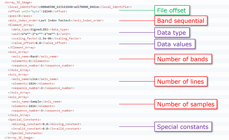
The label metadata contains some important information about the image (see the red boxes pointers):
- The image has 3 bands. We can tell from the axis_index_order and the sequence_number values that the image is in band sequential order because the last index (sample) changes fastest.
- The image has 1024 lines and 1024 samples per line.
- Pixel values are stored using the SignedLSB2 data type. Numbers for this data type are two-byte integers in least significant byte order.
The label gives some additional info (purple and green box pointers):
- The file offset value tells us that the data file contains 10,240 bytes of non-image data before the start of the image. You may need to enter this value into your software program when reading the image. Note that the offset is in bytes—the data type doesn't matter to the offset.
- The image data type is SignedLSB2, meaning signed two's complement two-byte integer with the least significant bit first. PDS allows a large handful of data types out of the roughly bajillion available data types. Your computer program should know what to do with this knowledge, but if you aren't sure, contact us and we'll be glad to help!
- Other values in the example's "Element_array" include a unit of measure applicable to the data values, along with a scaling factor and offset. These last two numbers, when present, should be applied to each pixel value in the image to get the actual data value for the pixel.
- Finally, special constants may be given. They aren't applicable for this particular image, but imagine a case when an instrument error results in some of the image being invalid. Employing a special constant informs the user that pixels with a certain value, for example -999, are invalid.
All archive images have metadata that describe the image structure.
Working with images inside the Notebook
The Notebook presents image data in several ways.
-
Image thumbnails show up in lots of places: the Sol summaries, search results, your user history, popup windows and the like. In some cases, the thumbnails shown are not created from the particular type of product being referenced. For example, if you are looking at an XYZ data product that contains pixel locations on the planet surface, the thumbnail will be from the companion visible spectrum image. You can read more about product types in Understanding data products.
-
Browse images are displayed when a product detail page is opened. These images are resampled to a lower resolution when the original is larger (in pixels) than the display window. The resampling negatively impacts the image quality. Even when images are not resampled, the browse image is there to give you a general idea of the image. Full-resolution browse (JPEG and PNG) images are sometimes available for download from the product detail page or as a default option in the Cart settings. However you consume browse images, the source data product should be used for science.
-
Quick view is an option to look at full-resolution browse images with pan and zoom controls. When available, you can access Quick view from a product's detail window. As you might expect, these are not science quality data.
-
Image tool is a tool within the Notebook that lets you look at images and make annotations. For some images, measurement tools (location, distance, and profile) are available. The measurement tools are available only for mosaics and stereo image pairs that have corresponding XYZ data.
Working with images outside of the Notebook
Whether you work with the data as archived or with a browse version depends on what you are trying to do. Recall that a browse image is sufficient for tasks like learning the context of an observation, but in other cases, like radiometric studies, you must work with the original data. Some image data files do not make much sense as browse images, for example, reachability maps and XYZ location images.
Browse versions of images as JPEGs or PNGs are available from the Notebook in two ways. When viewing an image product in the detail window, select Action > Download from the menu. In addition to the archived image and its label, browse versions will be listed and may be downloaded individually. To get browse versions of multiple images, add the images to the cart. Then, at checkout, edit your settings to include a browse image with your order. These browse images can be viewed by any software that reads JPEG or PNG images.
More specialized software is required for images in PDS format. These packages need to have a built-in reader that understands PDS format, or allow you the opportunity to input image parameters from the label. Available packages include:
- Free
- The PDS View is a general visualization tool that can read all types of PDS4 data. [https://github.com/NASA-PDS/pds-view]
- The PDS Transform tool is a Java-based command-line tool for transforming PDS3 and PDS4 product labels and data into other formats. [https://nasa-pds.github.io/transform/]
- GDAL is a translator library for raster and vector geospatial data formats. [https://gdal.org/]
ISIS is the USGS software package designed to ingest and manipulate image data from past and current NASA and many international planetary missions that have visited bodies in the Solar System. [https://isis.astrogeology.usgs.gov/]
- Commercial
- ESRI ArcGIS supports some PDS images natively with the option to manually enter format details.
- Harris Geospatial ENVI/IDL supports some PDS images natively with the option to manually enter format details.
- MathWorks MATLAB can be used for numeric processing of image data. Format details must be manually entered.
The document at https://pds-geosciences.wustl.edu/documents/ViewingPDSImagesAndExportingToOtherFormats.pdf gives examples of using some of these tools.